
Table of Contents
ToggleBy the end of this lecture, you should be able to:
- Define probability and apply simple probability rules in health examples.
- Recognise a normal distribution and explain why it matters in statistics.
- Compute a z-score and explain whether a value is typical or unusual.
- Calculate and interpret 95% confidence intervals for means and proportions.
- Communicate statistical uncertainty in plain, correct language.
🎯 The Big Picture: Health data are often incomplete samples. We cannot measure every patient in the country. Probability helps us describe how much uncertainty remains when we use sample results to understand a wider population. The journey is:
Probability is the language of uncertainty. In nursing and public health, we rarely deal with absolute certainties. A test may be "likely" positive. A patient may be "at risk" of complications. Probability gives us a number to express that uncertainty.
| Term | Definition | Nursing Example |
|---|---|---|
| Outcome | One possible result of a process. | A malaria RDT result is positive. |
| Event | A group of one or more outcomes. | The patient has malaria (could be confirmed by RDT, microscopy, or clinical signs). |
| Probability | A number from 0 to 1 showing how likely an event is. | There is a 0.30 (30%) chance that a mother will book ANC before 12 weeks. |
Probability = Number of Favourable Outcomes ÷ Total Possible Outcomes
Example: If 30 out of 100 mothers attend ANC before 12 weeks, the probability is 30 ÷ 100 = 0.30 = 30%.
Three essential rules every nurse should use correctly when interpreting health data:
Probability cannot be below 0 or above 1.
- 0 = Impossible (e.g., the probability that a living patient has a negative heart rate).
- 1 = Certain (e.g., the probability that a patient who has died will not recover).
- 0.5 = 50/50 chance (e.g., a coin flip — though health probabilities are rarely this neat).
If an event either happens or does not happen, the probabilities must add to 1.
P(not A) = 1 − P(A)
Example: If P(malaria) = 0.25 in a community, then P(no malaria) = 1 − 0.25 = 0.75 (or 75%).
Why this matters: If you know 15% of patients have hypertension, you immediately know 85% do not. This is useful for planning resources and understanding risk.
For non-overlapping (mutually exclusive) events, you can add their probabilities:
P(A or B) = P(A) + P(B)
Example: In a ward, the probability a patient has malaria is 0.20, and the probability a patient has typhoid is 0.10. Assuming no patient has both, the probability a random patient has either malaria or typhoid is 0.20 + 0.10 = 0.30 (30%).
A midwife reviews ANC attendance records at a health centre. Out of 150 mothers who registered for ANC:
| ANC Attendance Status | Number of Mothers | Probability |
|---|---|---|
| Attended first ANC before 12 weeks | 45 | 45/150 = 0.30 |
| Attended first ANC at 12 weeks or later | 105 | 105/150 = 0.70 |
| Total | 150 | 1.00 |
- Interpretation: In this clinic sample, the probability that a randomly selected mother booked ANC before 12 weeks is 0.30, or 30%.
- Complement Check: P(late ANC) = 1 − P(early ANC) = 1 − 0.30 = 0.70. This matches the table — a good way to verify your calculations.
- Clinical Application: If only 30% of mothers book early, the nurse manager knows that 70% are at higher risk for complications. This data supports an intervention: community health worker outreach, transport vouchers, or male partner involvement programs.
🩺 Scenario: In a village of 200 children under five, a nurse finds:
- 140 are fully immunised.
- 40 are partially immunised.
- 20 are unimmunised.
- P(fully immunised) = 140/200 = 0.70 (70%)
- P(partially immunised) = 40/200 = 0.20 (20%)
- P(unimmunised) = 20/200 = 0.10 (10%)
- P(not fully immunised) = 1 − 0.70 = 0.30 (30%) using the complement rule.
- P(either partially immunised OR unimmunised) = 0.20 + 0.10 = 0.30 (30%) using the addition rule (mutually exclusive).
Action: The 30% gap is a public health priority. The nurse can now argue for a catch-up campaign with precise numbers.
The normal distribution is a bell-shaped pattern found in many biological and health measurements. It is one of the most important concepts in statistics because it allows us to make predictions about what is "normal" and what is "unusual."
- Symmetric around the mean — the left side is a mirror image of the right side.
- Mean, median, and mode are all at the exact centre of the curve.
- Most values cluster near the mean. The curve is highest in the middle.
- Fewer values appear at the extremes. The "tails" get thinner as you move away from the centre.
- The total area under the curve equals 1 (or 100%), representing all possible outcomes.
- Adult height in a homogeneous population.
- Birth weight of full-term babies.
- Systolic blood pressure in a healthy adult population.
- Haemoglobin levels in non-anaemic adults.
- Examination scores in a large class.
| Application | Why It Matters |
|---|---|
| Clinical Measurement | A value can be compared with the expected average. Example: a baby with birth weight 2.1 kg can be compared to the population mean of 3.0 kg. Is this baby unusually small? |
| Sampling Distribution | Even if individual data are not normal, the means of many samples tend to form a normal pattern — especially when the sample size is large (Central Limit Theorem). This is why we can use normal-based formulas for confidence intervals. |
| Confidence Intervals | Normal theory helps us estimate how far a sample result (like a mean) may be from the true population value. It quantifies our uncertainty. |
📝 Exam Tip: When asked "Why does the normal distribution matter?" mention at least two of these three: clinical comparison, sampling distribution, and confidence intervals.
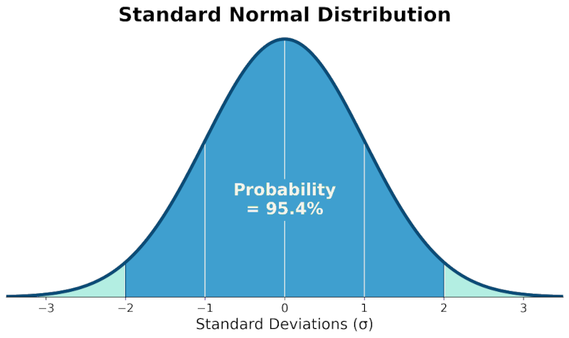
For any data that follows a normal distribution, the spread of values follows a remarkably predictable pattern:
- 68% of values fall within 1 SD of the mean
- 95% of values fall within 2 SD of the mean
- 99.7% of values fall within 3 SD of the mean
Mnemonic: "68, 95, 99.7 — Almost All Are Near the Middle"
What this means practically: If you know the mean and standard deviation of a normally distributed measurement, you can immediately say what range covers "most" patients, and you can flag values that are unusually high or low.
Systolic blood pressure is measured in a ward. The data are approximately normally distributed with:
- Mean (μ) = 120 mmHg
- Standard Deviation (SD) = 10 mmHg
| Range | Calculation | Approx. % of Patients |
|---|---|---|
| 110 to 130 mmHg | 120 ± 1 SD | 68% |
| 100 to 140 mmHg | 120 ± 2 SD | 95% |
| 90 to 150 mmHg | 120 ± 3 SD | 99.7% |
- Interpretation: A patient with systolic BP of 150 mmHg is about 3 SD above the mean. Only about 0.15% of patients in this population would be expected to have BP this high or higher. This patient should be considered unusually high and requires closer clinical attention — possibly immediate intervention.
- Conversely: A patient with BP of 115 mmHg is within 1 SD of the mean. This is typical and expected. No alarm needed.
🩺 Scenario: Birth weights in a district hospital are normally distributed with mean = 3.2 kg and SD = 0.5 kg.
- 68% of babies weigh between 2.7 kg and 3.7 kg (3.2 ± 0.5).
- 95% of babies weigh between 2.2 kg and 4.2 kg (3.2 ± 1.0).
- 99.7% of babies weigh between 1.7 kg and 4.7 kg (3.2 ± 1.5).
Clinical Application: A baby born at 1.8 kg is below the 3 SD lower limit. This is extremely unusual and signals possible prematurity, intrauterine growth restriction, or maternal malnutrition. The nurse should flag this immediately for paediatric review. A baby at 3.0 kg is well within the normal range — routine care is appropriate.
A z-score (also called a standard score) tells us how many standard deviations a particular value is from the mean. It converts any measurement into a common scale, allowing comparison across different variables.
z = (Observed Value − Mean) ÷ Standard Deviation
z = (x − μ) ÷ σ
| Z-Score | Meaning | Health Interpretation |
|---|---|---|
| z = 0 | Exactly at the mean. | Typical, average value. No concern. |
| z = +1 | 1 SD above the mean. | Higher than average, but still common (about 16% of population is above this). |
| z = −1 | 1 SD below the mean. | Lower than average, but still common (about 16% of population is below this). |
| z = +2 or more | 2 or more SD above the mean. | Unusually high. Only ~2.5% of population is above this. May need investigation. |
| z = −2 or less | 2 or more SD below the mean. | Unusually low. Only ~2.5% of population is below this. Often a clinical red flag. |
📝 Exam Tip: A z-score changes different measurements into a common scale. This means you can compare a baby's birth weight z-score with another baby's haemoglobin z-score, even though the original units (kg vs. g/dL) are completely different.
A baby is born with a birth weight of 2.1 kg. In the population, the mean birth weight is 3.0 kg with a standard deviation of 0.45 kg.
- z = (2.1 − 3.0) ÷ 0.45
- z = −0.9 ÷ 0.45
- z = −2.0
Interpretation: The baby's birth weight is 2 standard deviations below the mean. According to the empirical rule, only about 2.5% of babies would be expected to weigh this little or less. This is unusually low and may require closer clinical attention — kangaroo mother care, warming, feeding support, and possible referral.
Why z-scores matter in nursing: Instead of just saying "the baby is small," the nurse can say "the baby is 2 SD below the population mean." This is precise, comparable across hospitals, and immediately communicates severity to doctors and referral facilities.
🩺 Scenario: Two babies are born at the same hospital:
- Baby A: Birth weight = 2.5 kg. Population mean = 3.0 kg, SD = 0.5 kg.
- Baby B: Birth weight = 2.8 kg. Population mean = 3.5 kg, SD = 0.4 kg.
- Baby A: z = (2.5 − 3.0) ÷ 0.5 = −1.0 (1 SD below mean — somewhat small, but common).
- Baby B: z = (2.8 − 3.5) ÷ 0.4 = −1.75 (1.75 SD below mean — more unusually small for their population).
Conclusion: Even though Baby B weighs more in absolute terms (2.8 kg vs. 2.5 kg), Baby B is more unusually small relative to their population. This is why z-scores are powerful — they allow fair comparison across different groups.
In real-world nursing and public health, we almost never measure the entire population. We take a sample and use it to estimate what is true for the whole population. But samples are imperfect — they contain sampling error.
| Term | Definition & Example |
|---|---|
| Point Estimate | A single number from the sample that estimates the population value. Example: The sample mean haemoglobin is 11.2 g/dL. This is our best guess for the population mean — but it is probably not exactly right. |
| Sampling Error | The natural, unavoidable difference between a sample result and the true population value. If you took a different sample of 50 mothers, the mean Hb would likely be slightly different. This is NOT a mistake — it is expected variation. |
| Confidence Interval (CI) | A range of plausible values for the true population value. Instead of saying "the mean is 11.2," we say "the true mean is plausibly between 10.8 and 11.6." This makes uncertainty visible and honest. |
Use this when your outcome is numerical (continuous data) — for example, average birth weight, average waiting time, average haemoglobin level.
95% CI = mean ± 1.96 × (SD ÷ √n)
95% CI = mean ± 1.96 × SE
- Mean (x̄): The average calculated from your sample.
- SD (standard deviation): How much individual values vary around the mean.
- n (sample size): The number of people or observations in your sample.
- SE (standard error): SD ÷ √n. This measures the uncertainty around the sample mean. It tells us how far sample means typically vary from the true population mean.
- 1.96: The "multiplier" from the normal distribution that gives us approximately 95% confidence. (For 90% CI, use 1.645. For 99% CI, use 2.576.)
📝 Exam Tip — The Magic Number 1.96: For a 95% confidence interval, always use 1.96 (or approximately 2 for quick mental calculations). This number comes from the normal distribution: 95% of the area under the curve lies within 1.96 standard deviations of the mean.
A hospital quality improvement team wants to know the average length of stay for pneumonia patients. They review 64 patient records.
- n = 64 patients
- Mean stay = 4.2 days
- SD = 1.6 days
- Calculate SE: SE = SD ÷ √n = 1.6 ÷ √64 = 1.6 ÷ 8 = 0.20 days
- Calculate Margin of Error: 1.96 × SE = 1.96 × 0.20 = 0.39 days
- Calculate 95% CI: 4.2 ± 0.39
- Result: 95% CI = 3.81 to 4.59 days
Interpretation: We are 95% confident that the true mean length of stay for all pneumonia patients at this hospital (not just the 64 sampled) is between 3.81 and 4.59 days.
- A narrow interval (like 4.1 to 4.3 days) suggests a precise estimate — we have a good idea of the true value.
- A wide interval (like 2.5 to 6.0 days) suggests more uncertainty — we need more data or the variation is very high.
- How to make the interval narrower: Increase the sample size (n). The larger your sample, the more precise your estimate. This is why SE = SD ÷ √n — as n gets bigger, the denominator gets bigger, so SE gets smaller.
This is where many students lose marks in exams. The wording matters.
- "The data are consistent with a true mean between 3.81 and 4.59 days."
- "We are 95% confident that the true population mean lies between 3.81 and 4.59 days."
- "The plausible range for the true mean is 3.81 to 4.59 days."
- "There is a 95% chance that this exact interval contains the true mean." — Wrong! The true mean is fixed. The interval either contains it or it doesn't. The 95% refers to the METHOD, not this specific interval.
- "95% of patients stay between 3.81 and 4.59 days." — Wrong! The CI is about the MEAN, not individual patients. Individual stays vary much more widely.
- "The true mean is definitely between 3.81 and 4.59 days." — Wrong! There is still a 5% chance the true mean falls outside this range.
Use this when your outcome is categorical (yes/no, present/absent, positive/negative) — for example, the proportion of children immunised, the proportion of mothers satisfied with care, the proportion of patients testing positive for malaria.
95% CI = p ± 1.96 × √[ p(1 − p) ÷ n ]
- p: The sample proportion (as a decimal). Example: if 72 out of 120 children are immunised, p = 72/120 = 0.60.
- (1 − p): The complement of the proportion. Example: if p = 0.60, then 1 − p = 0.40 (the proportion NOT immunised).
- n: The total sample size.
- √[ p(1 − p) ÷ n ]: The standard error (SE) for a proportion.
⚠️ Critical Caution: When calculating a CI for a proportion, you MUST use decimals (0.60), not percentages (60%), inside the formula. Only convert back to percentages at the very end for your final interpretation.
A nursing student surveys immunisation coverage in a village. Out of 120 children under five, 72 were fully immunised.
- n = 120 children
- Number immunised = 72
- p = 72 ÷ 120 = 0.60
- Calculate SE: SE = √[ p(1 − p) ÷ n ] = √[ 0.60 × 0.40 ÷ 120 ]
- SE = √[ 0.24 ÷ 120 ] = √0.002 = 0.0447
- Calculate Margin: 1.96 × 0.0447 = 0.0876
- Calculate 95% CI: 0.60 ± 0.0876
- Result: 95% CI = 0.512 to 0.688 = 51.2% to 68.8%
Interpretation: We are 95% confident that the true immunisation coverage in the entire village (not just the 120 sampled children) is between 51.2% and 68.8%.
- The sample size (n = 120) is moderate. If we surveyed 500 children, the interval would be much narrower.
- The proportion (0.60) is in the middle — proportions near 0.50 have the largest standard errors.
- Clinical/Public Health Action: Even the upper bound (68.8%) is below the national target of 90%. This confirms that immunisation coverage is inadequate and justifies a catch-up campaign.
The first step is always to identify your outcome type. This determines which formula to use.
| Research Question | Outcome Type | Use This CI |
|---|---|---|
| What is the average birth weight? | Numerical (continuous) | CI for a mean |
| What proportion delivered in a facility? | Yes/No (categorical) | CI for a proportion |
| What is the average waiting time? | Numerical (continuous) | CI for a mean |
| What proportion tested malaria-positive? | Yes/No (categorical) | CI for a proportion |
📝 Quick Check:
- Mean = average amount (kg, minutes, g/dL, mmHg) ➔ Use CI for a mean.
- Proportion = share of people with a characteristic (%, fraction) ➔ Use CI for a proportion.
Mnemonic: "Means are Measured; Proportions are People."
A health centre records 50 postnatal mothers.
- Mean waiting time = 36 minutes, SD = 14 minutes.
- 32 mothers report satisfaction with services.
- SE = 14 ÷ √50 = 14 ÷ 7.071 = 1.98
- Margin = 1.96 × 1.98 = 3.88
- 95% CI = 36 ± 3.88 = 32.1 to 39.9 minutes
- p = 32/50 = 0.64 (64%)
- SE = √[0.64 × 0.36 ÷ 50] = √0.004608 = 0.0679
- Margin = 1.96 × 0.0679 = 0.133
- 95% CI = 0.64 ± 0.133 = 0.507 to 0.773 = 50.7% to 77.3%
Interpretation: The satisfaction estimate is less precise — the interval is fairly wide. With only 50 mothers, there is considerable uncertainty about the true satisfaction rate.
| Mistake | How to Fix It |
|---|---|
| Using percentages instead of decimals in proportion formulas. | Always convert 60% ➔ 0.60 before calculating. Convert back at the end. |
| Forgetting to divide SD by √n when calculating SE for a mean. | SE = SD ÷ √n. The √n is essential — it converts individual variation into uncertainty about the mean. |
| Interpreting a CI as a guarantee or a probability about one interval. | Say "we are 95% confident" or "the plausible range is." Do not say "95% chance." |
| Reporting only the p-value and hiding the confidence interval. | Always report the CI — it shows the size of the effect AND the precision. |
| Ignoring clinical context when deciding if a value is important. | A z-score of −1.9 may not be "statistically unusual" but may still need clinical action. |
- Probability: How likely is an event? Use counts ➔ convert to decimals.
- Normal Distribution: Bell-shaped. 68, 95, 99.7 rule. Most values near the mean.
- Z-Score: z = (x − mean) ÷ SD. Beyond ±2 = unusual. Common scale for comparison.
- Confidence Interval: Mean: x̄ ± 1.96×(SD/√n). Proportion: p ± 1.96×√[p(1−p)/n]. Shows precision.
- Probability: P = favourable ÷ total
- Complement: P(not A) = 1 − P(A)
- Z-score: z = (x − μ) ÷ σ
- SE for mean: SE = SD ÷ √n
- 95% CI for mean: mean ± 1.96 × SE
- SE for proportion: SE = √[p(1−p) ÷ n]
- 95% CI for proportion: p ± 1.96 × SE
- Rosner, B. (2015). Fundamentals of Biostatistics (8th ed.). Cengage Learning.
- Daniel, W. W., & Cross, C. L. (2018). Biostatistics: A Foundation for Analysis in the Health Sciences (11th ed.). Wiley.
- Gordis, L. (2013). Epidemiology (5th ed.). Saunders Elsevier.
- Heavey, E. (2018). Statistics for Nursing: A Practical Approach (3rd ed.). Jones & Bartlett Learning.
Quick Quiz
Probability, Normal Distribution and Confidence Intervals
Epidemiology and Biostatistics - mobile-friendly and focused practice.
Privacy: Your details are used only for quiz tracking and certificates.
Probability, Normal Distribution and Confidence Intervals
Epidemiology and Biostatistics
Preparing questions...
Choose your answer and keep your streak alive.
Great effort.
Here is your quick performance summary.