
By the end of this session, you should be able to:
- Explain the purpose of hypothesis testing in health research and nursing practice.
- Write clear null (H₀) and alternative (H₁) hypotheses for simple clinical questions.
- Use p-values and significance levels correctly without overclaiming.
- Select chi-square, paired t-test, or independent t-test appropriately based on data structure.
- Interpret test results in clear nursing and public health language — not just statistical jargon.
In real clinical and community practice, we rarely measure everybody. We take a sample a group of patients, a ward, a village and use that sample to make a careful, evidence-based judgement about the wider population.
Sample Result ➔ Statistical Test ➔ Evidence-Based Conclusion
- Hand Hygiene: Does a 2-hour hand hygiene training session improve compliance rates among student nurses on the maternity ward?
- Malaria Prevention: Is malaria positivity different between children who sleep under an insecticide-treated net and those who do not?
- Patient Education: Do mothers' knowledge scores about ORS preparation increase after a health education session?
- Clinic Efficiency: Is the average waiting time at Clinic A significantly shorter than at Clinic B?
- Nutrition: Is there an association between a child's sex and their nutritional status (wasted vs. not wasted)?
Statistical inference is the bridge between what we observe in our sample and what we believe is true in the entire population.
| Component | What It Is | Nursing Example |
|---|---|---|
| KNOWN Sample observed data | The actual numbers we collected from our study group. | We measured Hb levels in 120 pregnant mothers attending ANC at Hospital X. |
| METHOD Probability and tests | The mathematical rules (t-tests, chi-square, p-values) that judge whether our sample result is meaningful. | We run a statistical test to compare the mean Hb before and after iron supplementation. |
| UNKNOWN Population truth | The real situation in the entire population that we can never measure perfectly. | The true mean Hb among ALL pregnant mothers in the district, not just our 120. |
💡 Core Question of Inference: "Is the observed difference likely to be real, or could it be due to chance?"
A test does not prove truth; it measures how compatible the data are with the assumption of "no effect" (H₀). We are essentially asking: "If nothing were really happening, how surprised would I be to see these results?"
| Term | Simple Meaning | Nursing Example |
|---|---|---|
| Parameter | The true value in the entire population. Usually unknown. | The true mean haemoglobin (Hb) level among all pregnant mothers in Uganda. |
| Statistic | A value calculated from your sample data. This is what you actually know. | The mean Hb in the 120 mothers you actually tested at your clinic. |
| Sampling Error | The natural difference between a sample statistic and the true population parameter. It exists simply because we did not measure everyone. | Your sample mean Hb is 11.2 g/dL, but the true population mean might be 11.5 g/dL. That gap is sampling error. |
| Statistical Test | A formal mathematical rule for judging whether sample evidence is strong enough to support a conclusion. | Chi-square test, paired t-test, independent t-test, ANOVA. |
| Hypothesis | A clear, testable statement about a population that can be supported or refuted by data. | "Mothers who receive nutrition counselling have higher mean Hb than those who do not." |
Mnemonic: "Parameter = Population" and "Statistic = Sample". Both start with the same letter. If you know the whole population, it's a parameter. If you only have a sample, it's a statistic.
Every statistical test begins with a question. But a research question is usually written in plain English. To test it statistically, we must translate it into two formal statements: the null hypothesis (H₀) and the alternative hypothesis (H₁).
| Research Question | Null Hypothesis (H₀) | Alternative Hypothesis (H₁) |
|---|---|---|
| Does training improve knowledge scores among nurses? | Mean score before training = Mean score after training. (No difference) | Mean score before training ≠ Mean score after training. (There is a difference) |
| Is malaria positivity related to net use? | There is no association between net use and malaria positivity. | There is an association between net use and malaria positivity. |
| Do two clinics have different waiting times? | Mean waiting time in Clinic A = Mean waiting time in Clinic B. | Mean waiting time in Clinic A ≠ Mean waiting time in Clinic B. |
| Does iron supplementation reduce anaemia? | Mean Hb after supplementation = Mean Hb before supplementation. | Mean Hb after supplementation > Mean Hb before supplementation. |
| Is there a link between ward type and infection rate? | Ward type and infection rate are independent (no association). | Ward type and infection rate are associated. |
❌ Common Student Error: Writing H₀ as "The training will improve scores." That is actually H₁! H₀ must always be the "no effect / no difference / no association" statement. Think of H₀ as the skeptic's position — it assumes nothing interesting is happening until proven otherwise.
- It is the "no difference" or "no association" statement.
- It represents the status quo — what we would expect if chance alone were operating.
- We test H₀ because random variation can easily mislead us, especially with small samples.
- We never "prove" H₀ is true. We either reject it or fail to reject it.
- It is the statement the researcher thinks may be supported by evidence.
- It represents the new idea, the intervention effect, or the association we suspect.
- It is what we hope to find evidence for by finding evidence against H₀.
Think of H₀ as "innocent until proven guilty." The null hypothesis claims "nothing happened." Our data is the evidence. If the evidence is strong enough, we reject the claim of innocence (reject H₀). If the evidence is weak, we do not declare innocence — we simply say "not guilty enough to convict" (fail to reject H₀).
When we say a result is "statistically significant," we mean: "The data we observed would be very unlikely if H₀ were actually true." Therefore, we have reasonable grounds to doubt H₀ and consider H₁ instead.
✅ Correct: "We reject H₀" or "We fail to reject H₀."
❌ Incorrect: "We accept H₀" or "H₀ is true." — The test only tells us whether evidence is strong enough to discard H₀, not whether H₀ is definitively true.
| Type | Question It Answers | When to Use |
|---|---|---|
| Two-tailed | "Is there any difference?" (Could be higher OR lower) | Most classroom and research situations. Use this as your default. It tests for a difference in either direction. |
| One-tailed | "Is one group specifically higher or lower?" | Only when the direction is justified before analysis based on strong theory or prior evidence. E.g., "We expect training to increase scores, not decrease them." |
🛡️ Safe Rule for Students: Use a two-tailed test unless the study clearly planned a directional test before seeing the data. Never choose a one-tailed test just because it makes your p-value smaller — that is scientific misconduct.
Example: A new drug for hypertension might lower BP, raise BP, or do nothing. Since we are not sure of the direction, we use a two-tailed test. But if we are testing whether a proven anti-hypertensive drug reduces BP (and we have no reason to think it would raise it), a one-tailed test might be justified.
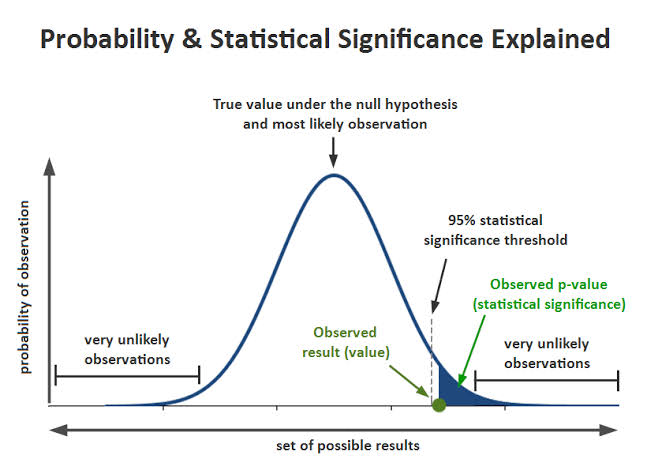
Alpha (α) is the cut-off point for deciding whether our evidence is strong enough to be called "statistically significant." It is the threshold of "surprise" — how unlikely must our results be under H₀ before we reject H₀?
α = 0.05
This means we are willing to accept a 5% chance of wrongly rejecting H₀ when it is actually true.
- If p ≤ 0.05: Reject H₀. The result is statistically significant. The evidence is strong enough to support H₁.
- If p > 0.05: Fail to reject H₀. The evidence is not strong enough. We do not have sufficient proof to support H₁.
⚠️ Critical Warning: α = 0.05 is a convention, not a law of nature. It is an arbitrary threshold agreed upon by scientists. A result with p = 0.051 is not magically "false," and p = 0.049 is not magically "true." The difference is tiny. Always interpret p-values as a continuum of evidence, not a binary switch.
A p-value is the probability of observing results as extreme as (or more extreme than) our sample result, assuming H₀ is true.
In plain nursing language: "If the intervention really did nothing, how lucky (or unlucky) would I have to be to see this result just by chance?"
| p-value | Statistical Interpretation | Nursing Language |
|---|---|---|
| p = 0.40 | Observed result is quite compatible with H₀. | "The difference we saw could easily happen by chance. No strong evidence of a real effect." |
| p = 0.06 | Evidence is suggestive, but not significant at α = 0.05. | "There is a hint of an effect, but we cannot be confident. Maybe the sample was too small." |
| p = 0.03 | Observed result is unlikely if H₀ is true. Reject H₀. | "This result would be surprising if the training had no effect. We have reasonable evidence it works." |
| p = 0.001 | Observed result is very unlikely if H₀ is true. Strong evidence. | "This would almost never happen by chance alone. We are very confident the effect is real." |
- They do NOT measure the probability that H₀ is true or false.
- They do NOT measure clinical importance or practical significance.
- They do NOT show the size of the effect (a tiny effect in a huge sample can have p < 0.001).
- They do NOT prove that the exposure caused the outcome — only that they are associated.
- They should ALWAYS be interpreted alongside confidence intervals, effect sizes, and study design.
Example: A drug lowers BP by 0.5 mmHg with p = 0.001. Statistically significant? Yes. Clinically important? No — no doctor would change practice for half a millimetre.
A confidence interval (CI) gives us a range of plausible values for the true population parameter. When combined with a p-value, it tells us both whether an effect exists and how large it might be.
| Result | How to Read It |
|---|---|
| Mean difference = 8.4 points, 95% CI: 7.0 to 9.8 | Likely improvement. The CI does not include 0, so the difference is statistically significant. We are 95% confident the true improvement is between 7.0 and 9.8 points. |
| Risk ratio = 1.20, 95% CI: 0.90 to 1.60 | Not statistically clear. The CI includes 1 (the "no effect" value for ratios), meaning the true effect could be no effect at all. The sample size may be too small. |
| Mean difference = 2.1 kg, 95% CI: −0.5 to 4.7 | Not significant. CI includes 0. The intervention might help a little, hurt a little, or do nothing. We cannot tell from this study. |
For differences (subtraction), "no effect" = 0. If the CI includes 0, the result is not significant.
For ratios (division), "no effect" = 1. If the CI includes 1, the result is not significant.
Mnemonic: "Difference = Zero, Ratio = One."
Because we are making decisions based on sample data (not the whole population), we can make mistakes. There are two types of errors we must understand:
| Reality | Your Decision | Error Name | Nursing Analogy |
|---|---|---|---|
| H₀ is true (No real effect) | You reject H₀ | Type I Error False Positive α = 0.05 | You think a new training works, but it actually doesn't. You waste resources rolling it out. |
| H₀ is false (Real effect exists) | You fail to reject H₀ | Type II Error False Negative β (beta) | You think a life-saving drug doesn't work, but it actually does. You deny patients effective treatment. |
Power = 1 − β. It is the probability that a study will correctly detect a real effect when one truly exists. Power improves when:
- Sample size is larger (more data = more precision).
- Measurement tools are accurate and reliable (less random noise).
- The true effect size is large (big differences are easier to detect).
- Variability in the data is low (consistent measurements).
Mnemonic: "Type I = Innocent person convicted" (false positive — you found an effect that isn't there).
Mnemonic: "Type II = Ignored criminal" (false negative — you missed an effect that is there).
Do not start by calculating. Start by understanding the data and the question. Follow this framework for every hypothesis test:
- Ask a clear question. What exactly are you trying to find out? Make it specific.
- State H₀ and H₁. Translate your question into formal null and alternative hypotheses.
- Choose α. Usually 0.05. Decide before you see the data.
- Select the right test. This depends on your data type and structure (see Section 12).
- Calculate the test statistic and p-value. Use software, calculator, or manual formulas.
- Interpret in context. Translate the numbers back into nursing or public health language.
QHATCI — "Quite Hard Always To Calculate, Initially"
The most common mistake students make is using the wrong test. The right test follows from two questions:
- What type of outcome variable do you have? (Categorical vs. Continuous)
- How many groups are you comparing, and are they related or independent?
| Outcome Variable | Groups / Comparison | Suitable Test | Nursing Example |
|---|---|---|---|
| Categorical (counts, proportions, yes/no) | Two categorical variables (association) | Chi-square (χ²) test | Is net use associated with malaria positivity? |
| Continuous (mean scores, weight, BP, time) | Same people measured twice (before/after) | Paired t-test | Did knowledge scores increase after training? |
| Continuous | Two separate, unrelated groups | Independent two-sample t-test | Is waiting time different in Clinic A vs. Clinic B? |
Used for relationships between two categorical variables.
- Tests whether two categorical variables are associated (linked) or independent (unrelated).
- Compares observed counts with the counts we would expect if H₀ were true.
- Useful for tables of frequencies — not means.
χ² = Σ (Observed − Expected)² / Expected
Sum across all cells in the table.
Research Question: Is sleeping under an insecticide-treated net (ITN) associated with malaria test result among febrile children?
- H₀: There is no association between net use and malaria test result.
- H₁: There is an association between net use and malaria test result.
Step 1: Observed Counts (Contingency Table)
| Net Use | Malaria Positive | Malaria Negative | Total |
|---|---|---|---|
| Yes (slept under net) | 18 | 42 | 60 |
| No (did not sleep under net) | 32 | 28 | 60 |
| Total | 50 | 70 | 120 |
The counts show fewer positive tests among children who slept under a net (18/60 = 30%) compared to those who did not (32/60 = 53.3%). But is this difference likely due to chance?
Step 2: Calculate Expected Counts
Formula: Expected count = (Row Total × Column Total) ÷ Grand Total
| Cell | Calculation | Expected Count |
|---|---|---|
| Yes & Positive | (60 × 50) ÷ 120 | 25 |
| Yes & Negative | (60 × 70) ÷ 120 | 35 |
| No & Positive | (60 × 50) ÷ 120 | 25 |
| No & Negative | (60 × 70) ÷ 120 | 35 |
Expected counts represent what we would see if net use and malaria were completely unrelated (H₀ true). Notice the totals still add up to 60 and 60.
Step 3: Calculate χ²
| Cell | Observed (O) | Expected (E) | O − E | (O − E)² | (O − E)² / E |
|---|---|---|---|---|---|
| Yes & Positive | 18 | 25 | −7 | 49 | 1.96 |
| Yes & Negative | 42 | 35 | +7 | 49 | 1.40 |
| No & Positive | 32 | 25 | +7 | 49 | 1.96 |
| No & Negative | 28 | 35 | −7 | 49 | 1.40 |
| Total χ² | 6.72 | ||||
Step 4: Interpretation
- χ² = 6.72, degrees of freedom (df) = 1, p ≈ 0.010.
- Since p = 0.010 ≤ 0.05, we reject H₀.
- Conclusion: Malaria test result is statistically associated with net use in this sample.
- Context wording: Children who slept under a net had lower observed malaria positivity (30% vs. 53.3%).
❌ Avoid saying: "Net use caused the lower malaria rate."
✅ Correct: "Net use was associated with lower malaria positivity." Causation requires stronger study designs (like RCTs), not just a chi-square test.
- Data are counts or frequencies, not percentages alone. (You can have percentages, but the test works on the raw counts behind them.)
- Categories are mutually exclusive: each person belongs in one cell only.
- Observations are independent — one person's result does not affect another's.
- Expected counts are generally at least 5 in most cells (some say 80% of cells). If not, use Fisher's exact test.
- Sample is collected in a way that represents the target population.
Scenario: A nurse investigates whether availability of handwashing stations at school is associated with diarrhoea among pupils.
| Handwashing Station | Diarrhoea: Yes | Diarrhoea: No | Total |
|---|---|---|---|
| Available | 12 | 48 | 60 |
| Not Available | 24 | 36 | 60 |
| Total | 36 | 84 | 120 |
Your Tasks:
- State H₀ and H₁.
- Calculate one expected count (e.g., Available & Yes).
- Decide whether chi-square is appropriate (check expected counts).
✅ Solution:
- H₀: There is no association between handwashing station availability and diarrhoea.
- H₁: There is an association between handwashing station availability and diarrhoea.
- Expected count (Available & Yes): (60 × 36) ÷ 120 = 18
- All expected counts: 18, 42, 18, 42 — all ≥ 5, so chi-square is appropriate.
- χ² calculation: (12−18)²/18 + (48−42)²/42 + (24−18)²/18 + (36−42)²/42 = 2.0 + 0.86 + 2.0 + 0.86 = 5.72
- Conclusion: p-value ≈ 0.017 (df=1). Since p < 0.05, reject H₀. Handwashing station availability is associated with diarrhoea risk.
Used when the same person is measured twice (before/after).
- Compares two related means.
- Common design: before-and-after measurement on the same participants.
- The test analyses the difference within each pair, not the raw scores.
- It answers: "Is the mean difference significantly different from zero?"
t = mean difference ÷ (SD of differences / √n)
Or simply: t = mean difference ÷ standard error of the difference
Paired data means the two measurements are linked or dependent. They are not independent observations.
| Paired Situation | Why It Is Paired |
|---|---|
| Knowledge score before and after training | Same learner measured twice. The "after" score depends on the "before" score. |
| Blood pressure before and after treatment | Same patient. Their baseline BP influences their post-treatment BP. |
| Left eye and right eye of same person | Two measurements linked to one individual's genetics and environment. |
| Mother's weight before and after nutrition counselling | Same mother. Her starting weight affects how much she can gain or lose. |
| Pain score before and after analgesia | Same patient. Their pain tolerance and condition are consistent across both measurements. |
Scenario: A nurse educator measures knowledge scores about infant nutrition before and after a 1-hour education session among 8 mothers.
The Raw Data
| Mother | 1 | 2 | 3 | 4 | 5 | 6 | 7 | 8 |
|---|---|---|---|---|---|---|---|---|
| Before | 45 | 50 | 55 | 60 | 52 | 48 | 58 | 62 |
| After | 55 | 58 | 63 | 70 | 59 | 56 | 64 | 72 |
| Difference (After − Before) | 10 | 8 | 8 | 10 | 7 | 8 | 6 | 10 |
Step-by-Step Calculation
- Calculate the mean difference:
Mean difference = (10 + 8 + 8 + 10 + 7 + 8 + 6 + 10) ÷ 8 = 67 ÷ 8 = 8.38 points - Calculate the standard deviation (SD) of the differences:
Using the formula for sample SD, SD of differences ≈ 1.51 - Calculate the standard error (SE) of the mean difference:
SE = SD / √n = 1.51 / √8 = 1.51 / 2.828 = 0.534 - Calculate the t-statistic:
t = mean difference / SE = 8.38 / 0.534 = 15.73 - Determine degrees of freedom and p-value:
df = n − 1 = 8 − 1 = 7. With t = 15.73 and df = 7, p < 0.001.
Interpretation
- Since p < 0.001 ≤ 0.05, we reject H₀.
- The mean increase in knowledge score (8.38 points) is statistically significant.
- Direction: Scores increased after health education. (Always state the direction!)
- Clinical context: The education session was effective at improving mothers' nutrition knowledge in this sample.
- The outcome variable is continuous or approximately continuous (e.g., scores, weight, BP).
- Pairs are genuinely linked: same person, matched pair, or before/after design.
- The differences are approximately normally distributed. (With n ≥ 30, this is less critical due to the Central Limit Theorem.)
- No extreme outliers in the differences. One wildly different pair can distort the mean.
- The measurement method is consistent before and after. (Don't change the scoring rubric mid-study!)
- ✅ Good Report: "Mean knowledge score increased from 53.8 before training to 62.1 after training. The mean paired increase was 8.38 points and was statistically significant, t(7) = 15.73, p < 0.001."
- ❌ Poor Report: "The training worked because p was less than 0.05."
Why it's poor: No means, no direction, no context. The reader has no idea how big the improvement was or whether it matters clinically.
Scenario: Eight patients have pain scores (0–10 scale) before and after counselling. The differences (After − Before) are: −2, −1, −3, 0, −2, −1, −4, −2.
Answer these:
- What is the outcome variable? Pain score (continuous, 0–10 scale).
- Why is a paired t-test appropriate? Same patient measured twice — before and after counselling.
- What does a negative difference mean? Pain score decreased after counselling. (Negative = After is lower than Before = improvement!)
- What would H₀ say? The mean difference in pain scores = 0 (counselling has no effect on pain).
- What would H₁ say? The mean difference ≠ 0 (counselling changes pain scores).
- Quick calculation: Mean difference = −1.875, SD ≈ 1.25, SE ≈ 0.44, t ≈ −4.26, p ≈ 0.004. Reject H₀. Counselling significantly reduced pain scores.
Used when comparing means from two separate, unrelated groups.
- Compares the mean of a continuous outcome in two independent groups.
- Independent means one participant belongs to only one group — there is no natural pairing.
- Example: Mean waiting time in Clinic A versus Clinic B.
- It asks: "Is the difference between group means larger than what we would expect by chance alone?"
| Question | Data Structure | Correct Test |
|---|---|---|
| Before and after training in the same learners | Same learners measured twice | Paired t-test |
| Clinic A patients vs. Clinic B patients | Different patients in two clinics | Independent t-test |
| Men vs. women Hb level | Different people in two groups | Independent t-test |
| Vaccinated children vs. unvaccinated children (immunity levels) | Two separate groups of children | Independent t-test |
| Mother's weight before and after nutrition program | Same mothers measured twice | Paired t-test |
Scenario: A district health officer wants to know if mean waiting time differs between Clinic A (new digital system) and Clinic B (paper-based system).
The Raw Data (waiting time in minutes)
| Clinic | Wait Times | |||||||
|---|---|---|---|---|---|---|---|---|
| Clinic A (Digital) | 40 | 45 | 50 | 42 | 48 | 46 | 44 | 47 |
| Clinic B (Paper) | 55 | 58 | 60 | 52 | 57 | 61 | 54 | 59 |
Descriptive statistics:
- Clinic A mean = 45.25 minutes
- Clinic B mean = 57.00 minutes
- Mean difference = 45.25 − 57.00 = −11.75 minutes
Inferential statistics:
- t ≈ −7.39
- df ≈ 14 (n₁ + n₂ − 2 = 8 + 8 − 2)
- p < 0.001
Decision: Since p < 0.05, we reject H₀. Mean waiting time differs significantly between the two clinics.
Context: Clinic B (paper-based) had significantly longer waiting times than Clinic A (digital). The digital system appears to improve patient flow.
- The outcome variable is continuous or approximately continuous.
- The two groups are independent — no person appears in both groups.
- The outcome is approximately normally distributed within each group. (Less critical with large samples, n > 30 per group.)
- No extreme outliers that would distort the mean.
- Variability (variance) in the two groups is reasonably similar. If not, use Welch's t-test (a modified version that handles unequal variances).
✅ Good Report: "Mean waiting time was 45.25 minutes in Clinic A and 57.00 minutes in Clinic B. The mean difference was −11.75 minutes and was statistically significant, t(14) = −7.39, p < 0.001."
Key addition: Always name the groups and the direction of the difference. Don't just say "significant" — say which group was higher/lower.
| Scenario | Correct Test | Why? |
|---|---|---|
| Sex of child vs. immunisation status (yes/no) | Chi-square | Two categorical variables. |
| Weight before and after nutrition counselling in same mothers | Paired t-test | Same people, before/after. |
| Mean Hb in two separate wards | Independent t-test | Two separate groups, continuous outcome. |
| Facility ownership (govt/private) vs. stock-out status (yes/no) | Chi-square | Two categorical variables. |
| Pain score before and after analgesia in same patients | Paired t-test | Same patients measured twice. |
| Mean BMI between urban and rural adolescents | Independent t-test | Two separate groups, continuous outcome. |
| Smoking status (yes/no) vs. TB status (yes/no) | Chi-square | Two categorical variables. |
| Knowledge scores of nurses trained online vs. nurses trained in-person | Independent t-test | Two different groups of nurses, continuous score. |
| Mistake | Why It Is Wrong | What To Do Instead |
|---|---|---|
| Using percentages instead of counts for chi-square | The formula requires raw counts. Percentages lose the sample size information. | Always construct the table with actual frequencies (n). |
| Using independent t-test for before-and-after data | You ignore the natural pairing, which increases error and reduces power. | Use a paired t-test when the same people are measured twice. |
| Reporting only p-values without means or proportions | A p-value tells you significance but not effect size or direction. | Always report means/SDs or proportions alongside p-values. |
| Claiming causation from a simple association | Association does not prove causation. Confounding variables may explain the link. | Use cautious language: "associated with," "linked to," not "caused." |
| Ignoring assumptions and outliers | Outliers can make means misleading. Non-normal data can invalidate t-tests. | Check your data first. Plot it. Look for outliers. Consider transformations or non-parametric tests. |
| Choosing α after seeing the p-value | This is data dredging / p-hacking. You are moving the goalposts. | Set α = 0.05 before any analysis. Stick to it. |
| Saying "accept H₀" when p > 0.05 | You never prove the null hypothesis. You only fail to find evidence against it. | Say "fail to reject H₀" or "no statistically significant difference was found." |
Scenario: A nurse educator measures infection prevention knowledge before and after a 2-hour training session among 20 student nurses. Scores range from 0 to 100.
Your Tasks & Solutions:
- Identify the outcome variable. Infection prevention knowledge score (continuous, 0–100).
- State H₀ and H₁.
- H₀: Mean knowledge score before training = Mean knowledge score after training.
- H₁: Mean knowledge score before training ≠ Mean knowledge score after training.
- Choose the most appropriate test. Paired t-test — same 20 nurses measured before and after.
- Explain why the test is appropriate. The data are continuous, and each participant serves as their own control. The two measurements are dependent (paired).
- Write one sentence showing how you would report a significant result.
"Mean infection prevention knowledge increased from 48.2 before training to 71.5 after training; the mean paired difference of 23.3 points was statistically significant, t(19) = 8.45, p < 0.001."
Complete the table. For each question, identify the data types and choose the correct test. Then justify your choice in one sentence.
| Question | Data Type | Test | Justification |
|---|---|---|---|
| Is nutrition status associated with sex? | Categorical + Categorical | Chi-square | Both variables are categories; we are testing association. |
| Did average temperature fall after treatment? | Continuous, paired | Paired t-test | Same patients measured before and after treatment. |
| Are mean ages different between two wards? | Continuous, independent | Independent t-test | Two separate groups of patients; age is continuous. |
| Is HIV testing uptake associated with age group? | Categorical + Categorical | Chi-square | Both uptake (yes/no) and age group (e.g., 15–24, 25–34) are categories. |
| Is mean blood pressure lower after a 6-month exercise program? | Continuous, paired | Paired t-test | Same hypertensive patients measured at baseline and 6 months. |
| Are recovery rates different between Hospital X and Hospital Y? | Categorical + Categorical | Chi-square | Recovery (recovered/not recovered) and hospital are both categorical. |
Cover the answers and test yourself. Use one clear sentence per answer.
- What does H₀ usually state?
Answer: H₀ states there is no difference, no association, or no effect — the "status quo" position. - What does p = 0.03 mean at α = 0.05?
Answer: The probability of seeing this result (or more extreme) if H₀ were true is 3%. Since 0.03 < 0.05, we reject H₀ and conclude a statistically significant result. - When do we use a chi-square test?
Answer: When we want to test whether two categorical variables are associated, using frequency counts in a contingency table. - What makes a t-test "paired"?
Answer: The same individual is measured twice (before/after), or two measurements are naturally linked (e.g., left eye and right eye). - Why should clinical meaning be reported alongside statistical significance?
Answer: A result can be statistically significant but clinically trivial (tiny effect in a huge sample), or clinically important but not significant (small sample). Both dimensions matter for patient care. - What is a Type I error?
Answer: Rejecting H₀ when it is actually true — a false positive. We think an effect exists when it does not. - What is a Type II error?
Answer: Failing to reject H₀ when it is actually false — a false negative. We miss a real effect. - What does a 95% confidence interval that includes 0 tell us about a mean difference?
Answer: The difference is not statistically significant at α = 0.05. The true effect could be zero.
The right statistical test follows the research question and the data structure. Do not memorise tests by topic — memorise them by variable type and group relationship.
- Categorical association (e.g., net use vs. malaria status) ➔ Chi-square test
- Same people before and after (e.g., knowledge scores pre/post training) ➔ Paired t-test
- Two separate groups with continuous outcomes (e.g., waiting time Clinic A vs. Clinic B) ➔ Independent t-test
- Always interpret in health context, not only by p-value.
- Always state the direction of the effect (which group was higher/lower).
- Never claim causation from a single test — say "associated with."
- Always check assumptions before choosing a test.
- Report means, SDs, and CIs alongside p-values.
- Polit, D. F., & Beck, C. T. (2020). Nursing Research: Generating and Assessing Evidence for Nursing Practice (11th ed.). Wolters Kluwer.
- Grove, S. K., & Gray, J. R. (2018). Understanding Nursing Research: Building an Evidence-Based Practice (7th ed.). Saunders.
- Field, A. (2018). Discovering Statistics Using IBM SPSS Statistics (5th ed.). SAGE Publications.
- Daniel, W. W., & Cross, C. L. (2018). Biostatistics: A Foundation for Analysis in the Health Sciences (11th ed.). Wiley.
Quick Quiz
Probability, Hypothesis Testing & Statistical Tests Quiz
Epidemiology and Biostatistics
Privacy: Your details are used only for quiz tracking and certificates.
Probability, Hypothesis Testing & Statistical Tests Quiz
Epidemiology and Biostatistics
Preparing questions...
Choose your answer and keep your streak alive.
Great effort.
Here is your quick performance summary.